Introduction - Working as part of delivery teams building, validating and delivering systems into production I quite appreciate the insight modelling tools provide and what one can achieve using that kind of insight. Understanding the various modelling techniques and knowing how to apply them allows for greater insight into the behavior of complex systems. Such insight gained can help with validation of sizing assumptions, un-realistic non-functional requirements and end user service level agreements (SLA’s) that the program might never be able to deliver on. Having the ability so pull together a few fundamentals equations to validate these critical assumptions at the design stage will save everyone a lot of trouble down the line.

The trick however is knowing what modelling techniques are appropriate for use and when. At the of the day any modelling technique is based on a bunch of assumptions that set the conditions within which the model is supposed to operate. So while modelling systems behavior to understand the system boundaries has great use, you should keep in mind the fact that there are many limitations in what these modelling techniques can really tell you. There’s no substitute for real world performance validation i.e. subjecting a system to real world conditions or through a simulated performance test with as realistic a workload as feasible. When that’s not feasible modelling the behavior of the system might be an option.

So based on past experience following are some of the delivery challenges which have led me down the path of modelling system behavior -

• Validation of key design assumptions early on
• Validation of key non functional requirements (NFR’s)
• Validation of growth in user workload (business forecasts) and their impact on capacity + user experience down the line
• Ability of the system to sustain growth in workload xx years down the line
• Validation of capacity sizing provided by vendors for a given workload
• Validation of performance testing results provided by 3rd parties and vendors

You can find many other scenarios where modelling systems behavior might be useful. At the end of day, keep in mind that any model you might use is just a bunch of equations based on a set of formal assumptions. So unless you are aware of what those assumptions are, the conditions the models can operate in and the limitations of the models you are using, you might end up creating a bigger trap for yourself. So tread wisely….:)

In this series of tutorials we will look at modelling system behavior using Dr. Neil Gunther’s PDQ (Pretty Damn Quick) Performance Analyser. Neil Gunther, (born 15 August 1950) is a computer information systems researcher best known internationally for developing the open-source performance modeling software Pretty Damn Quick and developing the Guerrilla approach to computer capacity planning and performance analysis. He has also been cited for his contributions to the theory of large transients in computer systems and packet networks, and his universal law of computational scalability. Gunther is a Senior Member of both the Association for Computing Machinery (ACM) and the Institute of Electrical and Electronics Engineers (IEEE), as well as a member of the American Mathematical Society (AMS), American Physical Society (APS), Computer Measurement Group (CMG) and ACM SIGMETRICS. You can read more about Dr. Neil Gunther here - Wikipedia.

Let’s Get Going With Pretty Damn Quick (PDQ) Analyzer - PDQ is an analytic solver library for queueing-network models (QNM) of computer systems, manufacturing systems, and data networks, that can be written optionally in a variety of conventional programming languages. Perl is the language used in the book Analyzing Computer System Performance with Perl::PDQ, which explains the fundamental queue-theoretic concepts with example PDQ models for computer performance analysis. PDQ (Pretty Damn Quick) is a downloadable free open source software package. If you are interested in picking up PDQ in further detail it’s recommended you pick up a copy of Dr. Neil Gunther’s book (link provided). Thanks to Dr. Gunther and his band of hackers, this fantastic modelling tool is free for everyone to make use of.

Here’s what Dr. Neil Gunther’s website has to say about PDQ. Link to website here : PDQ website - PDQ uses queue-theoretic paradigms to represent and solve all kinds of modern computer systems. Computer system resources (whether hardware and software) are represented by queues (more formally, a queueing network-not to be confused with a data network-which could be a PDQ queueing model) and the queueing model is solved “analytically” (meaning via a combination of algorithmic and numerical procedures). Queues are invoked as functions in PDQ by making calls to the appropriate library functions (listed below 3). Once the queueing model is expressed in PDQ, it can be solved almost instantaneously by calling the PDQ_Solve() function. This in turn generates a report of all the corresponding performance metrics such as: system throughput, and system response time, as well as details about queue lengths and utilizations at each of the defined queues. This algorithmic solution technique makes it orders of magnitude faster than setting up (and debugging; a step that is often not mentioned by simulationists) and running repeated (another step that is often glossed over) experiments to see if the solutions are statistically meaningful. PDQ solves everything as though it were in steady state. The tradeoff is that you cannot computer higher order statistics.

Analytic solvers are generally faster than simulators and this makes it ideal for the Performance-by-Design methodology described in the book. As part of its suite of solution methods, PDQ incorporates MVA (Mean Value Analysis) techniques. PDQ is not a hardwired application constrained to run only on certain personal computers. Instead, PDQ is provided as open source, written in the C language, to enable it to be used in the environment of your choice—from laptop to cloud. Moreover, PDQ is not a stand-alone application but a library of functions for solving performance models expressed as circuits or networks of queues. This also means that PDQ is available in a number of popular programming languages including C, Perl, Python and more recently, the R statistical language. You can read more at Link.

You’ll need access to a Linux virtual machine to be able to download, compile and run the Python version of PDQ which is covered in this tutorial. There are other versions of PDQ available and you are free to try them out instead. There’s no hard and fast rule that you need to stick with the Python version, we have used the Python version due to the fact that we simple love working with Python. You should pick the build of PDQ that works best for you and what you are trying to do.

Before you start, please make sure your virtual machine has a route to the internet. You can try pinging or resolving a remote IP address and confirm that you have connectivity. Once that’s resolved let’s move to the next step, which is downloading a copy of the PDQ repo. Please note that we are using the cutting edge version of PDQ but since it’s for purposes of this tutorial it doesn’t matter that much. You can go with a lower version if you aren’t comfortable using the cutting edge version. You will also note that all my installation commands are based on Ubuntu Linux. This might be different for you if you have a different version / distribution of Linux.

Issue the following command at your BASH console on the Linux virtual machine to create a local clone of the PDQ github repository.

bash# git clone https://github.com/DrQz/pdq-qnm-pkg.git

Once you’ve created a clone of the PDQ repository you are good to continue to the next step. Before we do anything else we’ll confirm the version of Python available and also install some development libraries for Python. So let’s issue the following command to confirm the version of Python installed on your Linux virtual machine.

bash# python –version

The above commands returns the following on my Linux virtual machine -

python 2.7.6

As long as you have a 2.7.xx version of Python installed you should be fine. If you don’t you’ll need to make sure you install Python 2.7 using the following command -

bash# sudo apt-get install Python2.7

Now that the Python coast is clear let’s go ahead and install a much needed dependency i.e. the Python 2.7 static development libraries including headers required to compile PDQ. Let’s install them using the following command.

bash# sudo apt-get install python-dev

With the installation of the Python development libraries and headers out of the way we are good to proceed with the actuall compilation of PDQ. Let’s change (or cd when on Linux) into the PDQ directory and issue the following commands -

bash# sudo make all

if the above doesn’t work for you, you can just compile the Python version.

bash# sudo make Python

You should now have all the required PDQ libraries installed in your system path. You’ll also find a bunch of examples in the Python directory within the locally cloned PDQ repo. Would recommend you take time going through them.

A Simple Queueing Example Using Fundamental Equations - It’s likely that most of us experience some sort of queues each day of our lives and in most cases we’ve comed to accept them. Eg. queueing up to purchase a coffee, or queueing outside a movie theatre to purchase tickets, or probably just lining up at the grocery counter to pay for the groceries you have just purchased. The science of the study of queues is called Queueing Theory and in many ways was inveted by Anger Krarup Erlang. Queueing theory is the mathematical study of waiting lines, or queues. A queueing model is constructed so that queue lengths and waiting time can be predicted. Queueing theory is generally considered a branch of operations research because the results are often used when making business decisions about the resources needed to provide a service. Queueing theory has its origins in research by Agner Krarup Erlang when he created models to describe the Copenhagen telephone exchange. The ideas have since seen applications including telecommunication, traffic engineering, computing[2] and, particularly in industrial engineering, in the design of factories, shops, offices and hospitals, as well as in project management.

So let’s see what a queueing system might look like -

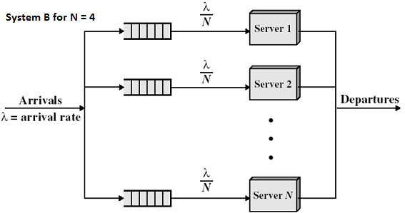
Let’s assume the above queueing system refers to a grocery store with customers arriving, getting serviced and then departing. In the above example we can see the customer arrivals at the store are denoted by Arrivals or letter λ. Let’s then assume the shoppers wander around the ailes, pick up the groceries they want, load them into their cart/trolley and then head over to one of the 4 counters. The counters or queues for the counters in this case is denoted by N. So in total N = 4. The arrival rate at each of the counters is then assumed to be λ/4 i.e. assuming equal balancing of incoming customers across each of the queues. Departures or completions is denoted by C or X (also called Throughput).

• Customers
  • The term customer in our case therefore represents queing of customers at the grocery checkout.
  • The customer in real life can also be equated to linux processes in a run queue
  • Messages waiting to be processed by a message router
  • Streaming media content (packets) being sent across the wire and queued up within the media processor
• Servers
  • The term server in our case refers to the cashier at the checkout counter
  • The server in real life could also mean the CPU or hardware processes which processes all the linux or unix processes
  • The server could also mean the hardware processes within a network router or switch processes incoming and outgoing messages.

In queueing theory, we refer to such a system as an M/M/1 queue, meaning that both arrival and service periods are memoryless or M (completely random in time) and there is only one server. Now, let’s calculate the properties of the M/M/1 queue by hand. To do this, we need to recall the relevant mathematical relations for the M/M/1 queue.

The quantities we will be dealing in our equations include the following -

• The average (Customer) arrival rate Lambda denoted by λ
• The average service time at the server denoted by S
• The average completion rate or throughput denoted by X
• The average customer wait time denoted by W
• The average customer response time denoted by R
• The average utilization of the system denoted by ρ

With all of that in the background the fundamental equations looks like -

• The average residence time a customer spends getting through the queueing system: R = S / (1 − λS).
• The utilization of the server: ρ = λS.
• The average queue length of the system: Q = λR.
• The average waiting time a customer can expect to spend before getting service: Wt = Rt − St (Response Time, Rt = Waiting Time, Wt + Service Time,St).

For the grocery store example we were looking at let’s now assume -

• Average arrival rate or Lamda is 0.25 per second or 1 every 4 seconds.
• Average customer service time is 1 seconds
• Number of cashiers in the store (system) is 1

The above system as we have mentioned before is called an M/M/1 system where both arrival and service periods are memoryless and there is only one server in the system.

Solving using the equations provided -

• Response time R = 1 / ( 1 - 0.25 * 1) = 1.33 seconds
• The utilization of the server: ρ = λS = 0.25 * 1 = 0.25 or 25%
• The average queue length of the system: Q = λR = 0.25 * 1.33 = 0.3325
• The average waiting time a customer can expect to spend before getting service: Wt = Rt − St = 1.33 - 1 = 0.333 seconds

So in summary for the above system we have Average (Customer) Response times = 1.33s, Utilization on the Server (checkout in our case) = 0.25 or 25%, Queue Length = 0.3325 and an average waiting time of ~1 second.

Re-visiting the Queuing Example Using PDQ - So let’s now build a python script using the examples provided by Dr. Gunther in the example directory of the PDQ code we’ve just downloaded. The script below is a modification of one such example provided. The input provided is similar to what we used in the above example.

• Average arrival rate or Lamda is 0.25 per second or 1 every 4 seconds.
• Average customer service time is 1 seconds
• Number of cashiers in the store (system) is 1

Here’s the script with the relevant parameters keyed into the script. To learn more about the functions used in the model below please read - PDQ Manual.

#!/usr/bin/python

import pdq

from math import *

arrivalRate = 0.25 # cust per sec

customerServiceTime = 1 # second

cashiers = 1

pdq.Init(“Grocery Store model”)

streams = pdq.CreateOpen(“Customers”, arrivalRate)

pdq.SetWUnit(“Cust”)

pdq.SetTUnit(“Sec”) # timebase for PDQ report

nodes = pdq.CreateNode(“Cashiers”, cashiers, pdq.MSQ)

pdq.SetDemand(“Cashiers”, “Customers”, customerServiceTime)

pdq.Solve(pdq.CANON)

pdq.Report()

So save the Python script and make sure it has it’s execute bit set (bash# chmod +x scriptname.py). Execute the script at the command line using the following command -

bash# ./scriptname.py

The result from executing the model is as follow -

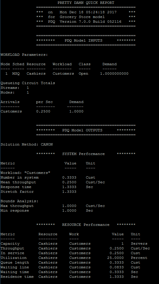
A review of the answers above suggest that they are very similar to the answers we’ve obtained using the fundamental equations. You can learn more about the fundamental equations here.

One can still use the fundamental equations for modelling behavior of simple systems but as systems start getting more complex i.e. multiple processors, multiple classes of workload, different types of systems i.e. transactions, batch, etc. use of PDQ modelling library really helps. The capability provided by PDQ simplifies creation of the different types of models and allows for quick analysis of system boundaries without having to perform complex math.

Conclusion - In this article we looked at the importance of modelling sytem constraints, the importance and relevance of Queueing Theory, Dr. Neil Gunther’s work and the awesome PDQ modelling library he’s given us, modelling system constraints for a Memoryless Single Server system using fundamental equations and finally modelling system constraints for Single Server Memoryless system using the PDQ library in Python. In our next article we will look at a more complex example of a bank where we have multiple classes of workload, multiple servers and multiple types of service demand from the customers. We’ll look at using PDQ to model system constraints for both transactional and batch systems.

Hope you have enjoyed this piece introducing the basic modelling concepts using fundamental equations and Dr. Gunthers Pretty Darn Quick modelling library. Head over to the SPE Fundamentals section to learn more about the fundamental equations and strengthen your understanding of the various related concepts.

Drop us a note if you have any questions, comments or input.